3.3 Notes on similarity solutions
The transient one dimensional heat equation may be represented: $$ \begin{equation} \frac{\partial T}{\partial \tau}=\alpha \frac{\partial^2 T}{\partial X^2} \tag{3.80} \end{equation} $$
where \( \tau \) and \( X \) denote time and spatial coordinates, respectively. The temperature \( T \) is a function of time and space \( T=T(X,\tau) \), and \( \alpha \) is the thermal diffusivity. (See appendix B in Numeriske Beregninger for a derivation)
Figure 42: Beam in the right half-space in one-dimension.

In Figure 42 a one-dimensional beam in the right half-space (\( 0\leq X < \infty \)) is illustrated. The beam has initially a temperature \( T_s \), but at time \( \tau=0 \), the temperature at the left end \( X=0 \) is abruptly set to \( T_0 \), and kept constant thereafter.
We wish to compute the temperature distribution in the beam as a function of time \( \tau \). The partial differential equation describing this problem is given by equation (3.80), and to model the time evolution of the temperature we provide the following initial condition: $$ \begin{equation} T(X,\tau)=T_s,\ \tau < 0 \tag{3.81} \end{equation} $$
along with the boundary conditions which do not change in time: $$ \begin{equation} T(0,\tau)=T_0,\ T(\infty,\tau)=T_s \tag{3.82} \end{equation} $$
Before we solve the problem numerically, we scale equation (3.80) by the introduction of the following dimensionless variables: $$ \begin{equation} u=\frac{T-T_0}{T_s-T_0},\qquad x=\frac{X}{L},\qquad t=\frac{\tau \cdot \alpha}{L^2} \tag{3.83} \end{equation} $$
where \( L \) is a characteristic length. By substitution of the dimensionless variables in equation (3.83) in (3.80), we get the following: $$ \begin{equation} \frac{\partial u}{\partial t}=\frac{\partial^2 u}{\partial x^2},\qquad 0 < x < \infty \tag{3.84} \end{equation} $$ accompanied by the dimensionless initial condition: $$ \begin{equation} u(x,t)=1,\quad t < 0 \tag{3.85} \end{equation} $$ and dimensionless boundary conditions: $$ \begin{equation} u(0,t)=0,\qquad u(\infty,t)=1 \tag{3.86} \end{equation} $$
The particular choice of the time scale in \( t \) (3.83) has been made to make the thermal diffusivity vanish and to present the governing partial on a canonical form (3.84) which has many analytical solutions and a wide range of applications. The dimensionless time in (3.83) is a dimensionless number, which is commonly referred to as the Fourier-number.
We will now try to transform the partial differential equation (3.84) with boundary conditions (3.85) to a simpler ordinary differential equations. We will do so by introducing some appropriate scales for the time and space coordinates: $$ \begin{equation} \bar{x}=a\, x \qquad \text{and} \qquad \bar{t}=b\, t \tag{3.87} \end{equation} $$
where \( a \) and \( b \) are some positive constants. Substitution of equation (3.87) into equation (3.84) yields the following equation: $$ \begin{equation} \frac{\partial u}{\partial \bar{t}}=\frac{a^2}{b}\frac{\partial^2u}{\partial \bar{x}^2} \tag{3.88} \end{equation} $$
We chose \( b=a^2 \) to bring the scaled equation (3.88) on the canonical, dimensionless form of equation (3.84) with the boundary conditions: $$ \begin{equation} u(x,t)=u(\bar{x},\bar{t})=u(ax,a^2t),\qquad \text{with} \quad b=a^2 \tag{3.89} \end{equation} $$
For (3.89) to be independent of \( a > 0 \), the solution \( u(x,t) \) has to be on the form: $$ \begin{equation} u(x,t)=f\left( \frac{x}{\sqrt{t}}\right),\ g\left( \frac{x^2}{t}\right),\ \text{etc.} \tag{3.90} \end{equation} $$
and for convenience we choose the first alternative: $$ \begin{equation} u(x,t)=f\left( \frac{x}{\sqrt{t}}\right) = f \left (\eta \right ) \tag{3.91} \end{equation} $$
where we have introduced a new similarity variable \( \eta \) defined as: $$ \begin{equation} \eta=\frac{x}{2 \sqrt{t}} \tag{3.92} \end{equation} $$
and the factor \( 2 \) has been introduced to obtain a simpler end result only. By introducing the similar variable \( \eta \) in equation (3.91), we transform the solution (and the differential equation) from being a function of \( x \) and \( t \), to only depend on one variable, namely \( \eta \). A consequence of this transformation is that one profile \( u(\eta) \), will define the solution for all \( x \) and \( t \), i.e. the solutions will be similar and is denoted a similarity solution for that reason and (3.92) a similarity transformation.
The Transformation in equation (3.92) is often referred to as the Boltzmann-transformation.
The original PDE in equation (3.84) has been transformed to an ODE, which will become clearer from the following. We have introduced the following variables: $$ \begin{equation} t=\frac{\tau\cdot\alpha}{L^2},\qquad \eta=\frac{x}{2 \sqrt{t}}=\frac{X}{2 \sqrt{\tau\alpha}} \tag{3.93} \end{equation} $$
Let us now solve equation (3.84) analytically and introduce: $$ \begin{equation} u=f(\eta) \tag{3.94} \end{equation} $$
with the boundary conditions: $$ \begin{equation} f(0)=0,\ f(\infty)=1 \tag{3.95} \end{equation} $$
Based on the mathematical representation of the solution in equation (3.94) we may express the partial derivatives occurring in equation (3.84) as: $$ \begin{align*} \frac{\partial u}{\partial t} & =\frac{\partial u}{\partial\eta}\left( \frac{\partial n}{\partial t}\right)=f'(\eta)\cdot\left( -\frac{x}{4t\sqrt{t}}\right)=-f'(\eta)\frac{\eta}{2t} \\ \frac{\partial u}{\partial x}&=\frac{\partial u}{\partial\eta}\left( \frac{\partial\eta}{\partial x}\right)=f'(\eta)\frac{1}{2\sqrt{t}},\qquad \frac{\partial^2u}{\partial x^2}=\frac{\partial}{\partial x}\left( f'(\eta)\frac{1}{2\sqrt{t}}\right)=f''(\eta)\frac{1}{4t} \end{align*} $$
By substituting the expressions for \( \dfrac{\partial u}{\partial t} \) and \( \dfrac{\partial^2u}{\partial x^2} \) in equation (3.84) we transform the original PDE in equation (3.84) to an ODE in equation (3.96) as stated above: $$ \begin{align*} f''(\eta)\frac{1}{4t}+f'(\eta)\frac{\eta}{2t}=0 \end{align*} $$
or equivalently: $$ \begin{equation} f''(\eta)+2\eta f'(\eta)=0 \tag{3.96} \end{equation} $$
The ODE in equation (3.96) may be solved directly by integration. First, we rewrite equation (3.96) as: $$ \begin{equation*} \frac{f''(\eta)}{f'(\eta)}=-2\eta\ \end{equation*} $$ which may be integrated to yield: $$ \begin{equation} \ln f'(\eta)=-\eta^2+\ln C_1 \tag{3.97} \end{equation} $$ which may be simplified by and exponential transformation on both sides: $$ \begin{equation*} f'(\eta)=C_1e^{-\eta^2} \end{equation*} $$ and integrated once again to yield: $$ \begin{equation} f(\eta)=C_1 \int_0^\eta e^{-t^2}\,dt \tag{3.98} \end{equation} $$
where we have used the boundary condition \( f(0)=0 \) from (3.95).
The integral in (3.98) is related with the error function: $$ \begin{equation*} \int_0^x e^{-t^2}dt=\frac{\sqrt{\pi}}{2} \text{erf(x)} \end{equation*} $$ where the error function \( erf(x) \) is defined as: $$ \begin{equation} \frac{2}{\sqrt{\pi}}\int_0^x e^{-t^2}dt \tag{3.99} \end{equation} $$
Substitution of equation (3.99) in equation (3.98) yields: $$ \begin{equation} f(\eta)=C_1\frac{\sqrt{\pi}}{2}\text{erf}(\eta ) \tag{3.100} \end{equation} $$
As the error function has the property \( \mathrm{erf(\eta)} \to 1 \) for \( \eta\to\infty \) we get: \( C_1=\dfrac{2}{\sqrt{\pi}} \) , and subsequent substitution of equation (3.100) yields:
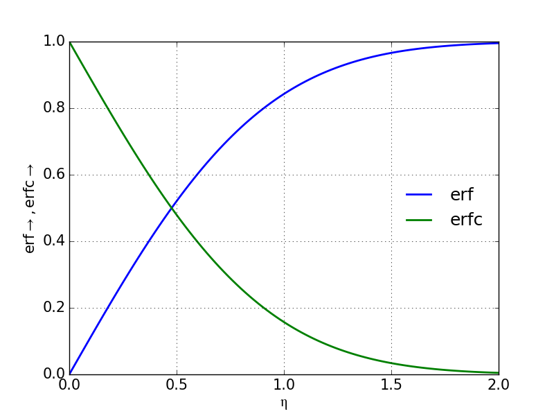
In Figure 43 the error function \( \text{erf}(\eta) \), which is a solution of the one-dimensional heat equation (3.84), is plotted along with the complementary error function \( \text{erfc}(\eta) \) defined as: $$ \begin{equation} \text{erfc}(\eta)=1-\text{erf}(\eta)=\frac{2}{\sqrt{\pi}}\int_{\eta}^\infty e^{-t^2} \;dt \tag{3.103} \end{equation} $$
Figure 43: The error function is a similarity solution of the one-dimensional heat equation expressed by the similarity variable \( \eta \).