2.6.6 Example: Falling sphere with constant and varying drag
We write (2.58) and (2.59) as a system as follows, $$ \begin{align} & \frac{dz}{dt}=v \tag{2.67}\\ & \frac{dv}{dt}=g-\alpha v^2 \tag{2.68} \end{align} $$ where $$ \begin{equation*} \alpha =\frac{3\rho _f}{4\rho _k\cdot d}\cdot C_D \end{equation*} $$ The analytical solution with \( z(0)=0 \) and \( v(0)=0 \) is given by $$ \begin{align} \tag{2.69} z(t)& =\frac{\ln(\cosh(\sqrt{\alpha g}\cdot t))}{\alpha} \\ v(t) &=\sqrt{\frac{g}{\alpha}}\cdot \tanh (\sqrt{\alpha g}\cdot t) \tag{2.70} \end{align} $$ The terminal velocity \( v_t \) is found by \( \displaystyle \frac{dv}{dt}=0 \) which gives \( \displaystyle v_t=\sqrt{\frac{g}{\alpha}} \).
We use data from a golf ball: \( d= 41\text{ mm} \), \( \rho_k = 1275 \text{ kg/m}^3 \), \( \rho_k = 1.22 \text{ kg/m}^3 \), and choose \( C_D = 0.4 \) which gives \( \alpha = 7\cdot 10^{-3} \). The terminal velocity then becomes $$ \begin{equation*} v_t = \sqrt{\frac{g}{\alpha}} = 37.44 \end{equation*} $$
If we use Taylor's method from the section 2.3 Taylor's method we get the following expression by using four terms in the series expansion: $$ \begin{align} \tag{2.71} z(t)=&\frac{1}{2}gt^2\cdot (1-\frac{1}{6}\alpha gt^2)\\ v(t)=&g t\cdot (1-\frac{1}{3}\alpha gt^2) \tag{2.72} \end{align} $$
By applying the Euler scheme (2.55) on (2.67) and (2.68) $$ \begin{align} \tag{2.73} z_{n+1}&=z_n+\Delta t\cdot v_n \\ v_{n+1}&=v_n+\Delta t\cdot (g-\alpha\cdot v^2_n),\ n=0,1,\dots \tag{2.74} \end{align} $$ with \( z(0)=0 \) and \( v(0)=0 \).
By adopting the conventions proposed in (2.23) and substituting \( z_0 \) for \( z \) and \( z_1 \) for \( v \) and we may render the system of equations in (2.67) and (2.68) as: $$ \begin{align*} & \frac{dz_0}{dt}=z_1 \\ & \frac{dz_1}{dt}=g-\alpha z_1^2 \end{align*} $$
One way of implementing the integration scheme is given in the following function euler():
def euler(func,z0, time):
    """The Euler scheme for solution of systems of ODEs.
    z0 is a vector for the initial conditions,
    the right hand side of the system is represented by func which returns
    a vector with the same size as z0 ."""

    z = np.zeros((np.size(time),np.size(z0)))
    z[0,:] = z0

    for i in range(len(time)-1):
        dt = time[i+1]-time[i]
        z[i+1,:]=z[i,:] + np.asarray(func(z[i,:],time[i]))*dt

    return z
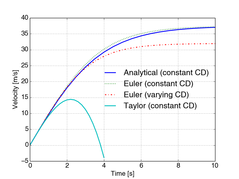
The program FallingSphereEuler.py computes the solution for the first 10 seconds, using a time step of \( \Delta t=0.5 \) s, and generates the plot in Figure 10. In addition to the case of constant drag coefficient, a solution for the case of varying \( C_D \) is included. To find \( C_D \) as function of velocity we use the function cd_sphere() that we implemented in (2.6.4 Example: Sphere in free fall). The complete program is as follows,
# src-ch1/FallingSphereEuler.py;DragCoefficientGeneric.py @ git@lrhgit/tkt4140/src/src-ch1/DragCoefficientGeneric.py;
from DragCoefficientGeneric import cd_sphere
from matplotlib.pyplot import *
import numpy as np

# change some default values to make plots more readable
LNWDT=2; FNT=11
rcParams['lines.linewidth'] = LNWDT; rcParams['font.size'] = FNT


g = 9.81      # Gravity m/s^2
d = 41.0e-3   # Diameter of the sphere
rho_f = 1.22  # Density of fluid [kg/m^3]
rho_s = 1275  # Density of sphere [kg/m^3]
nu = 1.5e-5   # Kinematical viscosity [m^2/s]
CD = 0.4      # Constant drag coefficient

def f(z, t):
    """2x2 system for sphere with constant drag."""
    zout = np.zeros_like(z)
    alpha = 3.0*rho_f/(4.0*rho_s*d)*CD
    zout[:] = [z[1], g - alpha*z[1]**2]
    return zout

def f2(z, t):
    """2x2 system for sphere with Re-dependent drag."""
    zout = np.zeros_like(z)
    v = abs(z[1])
    Re = v*d/nu
    CD = cd_sphere(Re)
    alpha = 3.0*rho_f/(4.0*rho_s*d)*CD
    zout[:] = [z[1], g - alpha*z[1]**2]
    return zout

# define euler scheme
def euler(func,z0, time):
    """The Euler scheme for solution of systems of ODEs.
    z0 is a vector for the initial conditions,
    the right hand side of the system is represented by func which returns
    a vector with the same size as z0 ."""

    z = np.zeros((np.size(time),np.size(z0)))
    z[0,:] = z0

    for i in range(len(time)-1):
        dt = time[i+1]-time[i]
        z[i+1,:]=z[i,:] + np.asarray(func(z[i,:],time[i]))*dt

    return z

def v_taylor(t):
#    z = np.zeros_like(t)
    v = np.zeros_like(t)

    alpha = 3.0*rho_f/(4.0*rho_s*d)*CD
    v=g*t*(1-alpha*g*t**2)
    return v

# main program starts here

T = 10  # end of simulation
N = 20  # no of time steps
time = np.linspace(0, T, N+1)

z0=np.zeros(2)
z0[0] = 2.0

ze = euler(f, z0, time)     # compute response with constant CD using Euler's method
ze2 = euler(f2, z0, time)   # compute response with varying CD using Euler's method

k1 = np.sqrt(g*4*rho_s*d/(3*rho_f*CD))
k2 = np.sqrt(3*rho_f*g*CD/(4*rho_s*d))
v_a = k1*np.tanh(k2*time)   # compute response with constant CD using analytical solution

# plotting

legends=[]
line_type=['-',':','.','-.','--']

plot(time, v_a, line_type[0])
legends.append('Analytical (constant CD)')

plot(time, ze[:,1], line_type[1])
legends.append('Euler (constant CD)')

plot(time, ze2[:,1], line_type[3])
legends.append('Euler (varying CD)')

time_taylor = np.linspace(0, 4, N+1)

plot(time_taylor, v_taylor(time_taylor))
legends.append('Taylor (constant CD)')

legend(legends, loc='best', frameon=False)
font = {'size' : 16}
rc('font', **font)
xlabel('Time [s]')
ylabel('Velocity [m/s]')
#savefig('example_sphere_falling_euler.png', transparent=True)
show()
Figure 10: Euler's method with \( \Delta t=0.5 \) s.