2.6 Euler's method
The ODE is given as $$ \begin{align} \tag{2.53} \frac{dy}{dx} = y'(x)&=f(x,y)\\ y(x_0)=&y_0 \tag{2.54} \end{align} $$ By using a first order forward approximation (2.29) of the derivative in (2.53) we obtain: $$ \begin{equation*} y(x_{n+1})=y(x_n)+h\cdot f(x_n,y(x_n))+O(h^2) \end{equation*} $$ or $$ \begin{equation} \tag{2.55} y_{n+1}=y_n+h\cdot f(x_n,y_n) \end{equation} $$ (2.55) is a difference equation and the scheme is called Euler's method (1768). The scheme is illustrated graphically in Figure 5. Euler's method is a first order method, since the expression for \( y'(x) \) is first order of \( h \). The method has a global error of order \( h \), and a local of order \( h^2 \).
Figure 5: Graphical illustration of Euler's method.

2.6.1 Example: Euler's method on a simple ODE
# src-ch1/euler_simple.py

import numpy as np
import matplotlib.pylab as plt

""" example using eulers method for solving the ODE
    y'(x) = f(x, y) = y
    y(0) = 1

    Eulers method:
    y^(n + 1) = y^(n) + h*f(x, y^(n)), h = dx
    """

N = 30
x = np.linspace(0, 1, N + 1)
h = x[1] - x[0] # steplength
y_0 = 1 # initial condition
Y = np.zeros_like(x) # vector for storing y values
Y[0] = y_0 # first element of y = y(0)

for n in range(N):
    f = Y[n]
    Y[n + 1] = Y[n] + h*f

Y_analytic = np.exp(x)

# change default values of plot to make it more readable
LNWDT=2; FNT=15
plt.rcParams['lines.linewidth'] = LNWDT
plt.rcParams['font.size'] = FNT

plt.figure()
plt.plot(x, Y_analytic, 'b', linewidth=2.0)
plt.plot(x, Y, 'r--', linewidth=2.0)
plt.legend(['$e^x$', 'euler'], loc='best', frameon=False)
plt.xlabel('x')
plt.ylabel('y')
#plt.savefig('../fig-ch1/euler_simple.png', transparent=True)
plt.show()
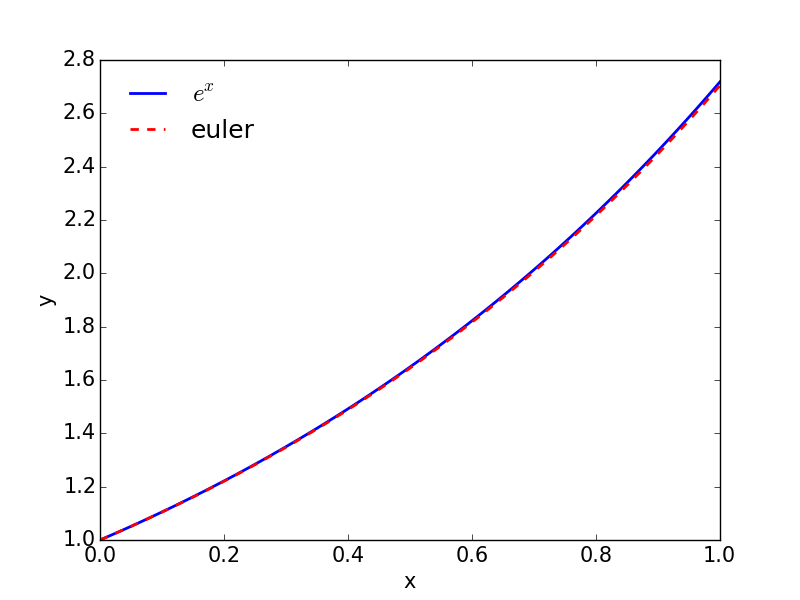
Figure 6: result from the code above
2.6.2 Example: Euler's method on the mathematical pendulum
# src-ch1/euler_pendulum.py

import numpy as np
import matplotlib.pylab as plt
from math import pi

""" example using eulers method for solving the ODE:
    theta''(t) + thetha(t) = 0
    thetha(0) = theta_0
    thetha'(0) = dtheta_0

    Reduction of higher order ODE:
    theta = y0
    theta' = y1
    theta'' = - theta = -y0

    y0' = y1
    y1' = -y0

    eulers method:
    y0^(n + 1) = y0^(n) + h*y1, h = dt
    y1^(n + 1) = y1^(n) + h*(-y0), h = dt
    """

N = 100
t = np.linspace(0, 2*pi, N + 1)
h = t[1] - t[0] # steplength
thetha_0 = 0.1
y0_0 = thetha_0 # initial condition
y1_0 = 0
Y = np.zeros((2, N + 1)) # 2D array for storing y values

Y[0, 0] = y0_0 # apply initial conditions
Y[1, 0] = y1_0

for n in range(N):
    y0_n = Y[0, n]
    y1_n = Y[1, n]

    Y[0, n + 1] = y0_n + h*y1_n
    Y[1, n + 1] = y1_n - h*y0_n

thetha = Y[0, :]
thetha_analytic = thetha_0*np.cos(t)

# change default values of plot to make it more readable
LNWDT=2; FNT=15
plt.rcParams['lines.linewidth'] = LNWDT
plt.rcParams['font.size'] = FNT

plt.figure()
plt.plot(t, thetha_analytic, 'b')
plt.plot(t, thetha, 'r--')

plt.legend([r'$\theta_0 \cdot cos(t)$', 'euler'], loc='best', frameon=False)
plt.xlabel('t')
plt.ylabel(r'$\theta$')
#plt.savefig('../fig-ch1/euler_pendulum.png', transparent=True)
plt.show()
Figure 7: result from the code above

2.6.3 Example: Generic euler implementation on the mathematical pendulum
# src-ch1/euler_pendulum_generic.py

import numpy as np
import matplotlib.pylab as plt
from math import pi

# define Euler solver
def euler(func, y_0, time):
    """ Generic implementation of the euler scheme for solution of systems of ODEs:
            y0' = y1
            y1' = y2
                .
                .
            yN' = f(yN-1,..., y1, y0, t)

            method:
            y0^(n+1) = y0^(n) + h*y1
            y1^(n+1) = y1^(n) + h*y2
                .
                .
            yN^(n + 1) = yN^(n) + h*f(yN-1, .. y1, y0, t)

        Args:
            func(function): func(y, t) that returns y' at time t; [y1, y2,...,f(yn-1, .. y1, y0, t)]
            y_0(array): initial conditions
            time(array): array containing the time to be solved for

        Returns:
            y(array): array/matrix containing solution for y0 -> yN for all timesteps"""

    y = np.zeros((np.size(time), np.size(y_0)))
    y[0,:] = y_0

    for i in range(len(time)-1):
        dt = time[i+1] - time[i]
        y[i+1,:]=y[i,:] + np.asarray(func(y[i,:], time[i]))*dt

    return y

def pendulum_func(y, t):
    """ function that returns the RHS of the mathematcal pendulum ODE:
        Reduction of higher order ODE:
        theta = y0
        theta' = y1
        theta'' = - theta = -y0

        y0' = y1
        y1' = -y0

        Args:
            y(array): array [y0, y1] at time t
            t(float): current time

        Returns:
            dy(array): [y0', y1'] = [y1, -y0]
        """

    dy = np.zeros_like(y)
    dy[:] = [y[1], -y[0]]
    return dy

N = 100
time = np.linspace(0, 2*pi, N + 1)
thetha_0 = [0.1, 0]

theta = euler(pendulum_func, thetha_0, time)
thetha = theta[:, 0]

thetha_analytic = thetha_0[0]*np.cos(time)

# change default values of plot to make it more readable
LNWDT=2; FNT=15
plt.rcParams['lines.linewidth'] = LNWDT
plt.rcParams['font.size'] = FNT

plt.figure()
plt.plot(time, thetha_analytic, 'b')
plt.plot(time, thetha, 'r--')

plt.legend([r'$\theta_0 \cdot cos(t)$', 'euler'], loc='best', frameon=False)
plt.xlabel('t')
plt.ylabel(r'$\theta$')
#plt.savefig('../fig-ch1/euler_pendulum.png', transparent=True)
plt.show()