7.3 Integral derivation of the 1D governing equations for a compliant vessel

7.3.1 1D transport equation

Figure 70: A compliant vessel with axial coordinate $ z $ and surface area $ A(z,t) $

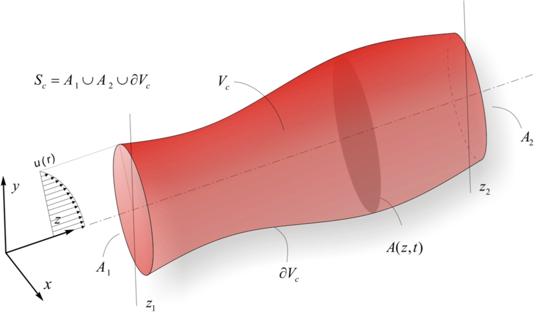
A fluid with constant mass density $ \rho $ is flowing through a compliant vessel of volume $ V_c $. The volume is bounded by two fixed spatial planes in the xy-plane, denoted $ A_1 $ and $ A_2 $, with corresponding coordinates $ z_1 $ and $ z_2 $. Vector components with respect to a fixed spatial coordinate system are denoted with subscripts 1, 2, 3, corresponding to respective spatial directions x, y, z, e.g., $ v_1, v_2, v_3 $ are the components of the velocity vector $ \boldsymbol{v} $. The lateral surface (luminary boundary) $ A $ of the vessel is allowed to move. However, note that it does not necessarily have to be a material surface with respect to the fluid, as fluid may be allowed to pass through the vessel wall [26]. Thus, the vessel volume $ V_c $, which we will consider as our control volume, has a surface $ S_c = A_1 \cup A_2 \cup A_3 $.

The Reynolds transport theorem for a moving control volume (2.33) with a generic density $ \beta $ takes the form: $$ \begin{equation} \tag{7.28} \dot{B} = \ddt \Int_{V(t)} \beta \, dV = \ddt \Int_{V_c(t)} \beta \, dV + \Int_{S_c(t)} \beta \, (\boldsymbol{v} -\boldsymbol{v}_c )\cdot \boldsymbol{n} \, dA \end{equation} $$ where $ \boldsymbol{v}_c $ denotes the velocity vector of the moving control volume $ V_c(t) $. In order to derive a 1D transport equation for a generic specific property, we will assume a particular controle volume $ V_c $, which is fixed in the axial direction (z-direction in figure 70), but follows the walls of the compliant vessel in the directions orthogonal to the chosen spatial direction (i.e., x- and y-directions in figure 70). By adopting the conventions of equation (2.26) a the more compact represenation of the RTT is obtained: $$ \begin{equation} \tag{7.29} \frac{dB}{dt} = \frac{dB_c}{dt} + \int_{S_c(t)} \beta (\boldsymbol{v} -\boldsymbol{v}_c) \cdot \boldsymbol{n} \, dA \end{equation} $$ The surface integrals may be simplified and split as $ S_c = A_1 \cup A_2 \cup A_3 $ and $ \boldsymbol{v}_c = 0 $ for all $ \boldsymbol{v}_c \in \{A_1,A_2\} $. By focusing on the first term of equation (7.29), we get from Leibniz's rule for 3D integrals (see equation (8.45)) or equation (2.32) for $ dB_c/dt $: $$ \begin{equation} \tag{7.30} \frac{dB_c}{dt} = \int_{V_c(t)} \partd{\beta}{t} \, dV + \int_{A_3} \beta \, \boldsymbol{v}_c \cdot \boldsymbol{n} \, dA \end{equation} $$ To simplify the integral in equation (7.30), we define an iterated them first in the direction which we want to express the spatial dependency and then in the orthogonal directions over which we will average: $$ \begin{equation} \tag{7.31} \Int_{V_c} (\cdot) \, dV = \Int_{z_1}^{z_2} \left \{ \Int_{A(x,t)} (\cdot) ,dA \right \} \, dz \quad \text{and} \quad \Int_{A_3} (\cdot)\, dA = \Int_{z_1}^{z_2} \left \{ \oint_{C(x,t)} (\cdot)\, dl \right \} \, dz \end{equation} $$ where $ C $ is the closed curve bounding $ A_3 $ orthogonal to the streamwise z-direction, and $ dl $ is the corresponding differential line element. Now, both integrals of equation (7.30) may be integrated along the z-axis: $$ \begin{equation} \tag{7.32} \frac{dB_c}{dt} = \int_{z_1}^{z_2} \left ( \int_{A_c} \partd{\beta}{t} \, dA + \oint_{C} \beta \, \boldsymbol{v}_c \cdot \boldsymbol{n} \, dl \right ) \, dz \end{equation} $$ Further, the cross-sectional mean value $ \bar{\beta} $ is defined conventionally as: $$ \begin{equation} \tag{7.33} \bar{\beta} = \frac{1}{A} \Int_{A} \beta \, dA \end{equation} $$ and for convenience we define $ B_s $: $$ \begin{equation} \tag{7.34} B_s \equiv A \bar{\beta} = \int_{A(t)} \beta dA \end{equation} $$ Based on the definitions in equation (7.34) we get from Leibniz's rule for 2D integrals (see equation (8.41)): $$ \begin{equation} \tag{7.35} \frac{dB_s}{dt} = \int_{A(t)} \partd{\beta}{t} \, dA + \oint_C \boldsymbol{v}_c \cdot \boldsymbol{n} \, dl = \ddt \left (A \bar{\beta} \right ) = \partd{A \bar{\beta}}{t} \end{equation} $$ The latter identity follows as this integral is valid for a fixed $ z $ only. This result in equation (7.35) may be substituted into equation (7.32) to yield: $$ \begin{equation} \tag{7.36} \frac{dB_c}{dt} = \int_{z_1}^{z_2} \partd{A \bar{\beta}}{t} \, dz \end{equation} $$

To proceed further, the surface integral of equation (7.29) may be split in the following manner: $$ \begin{equation} \tag{7.37} \Int_{S_c(t)} \beta \, (\boldsymbol{v} -\boldsymbol{v}_c )\cdot \boldsymbol{n} \, dA = \Int_{A_1} \beta \, (\boldsymbol{v} -\boldsymbol{v}_c )\cdot \boldsymbol{n}\, dA + \Int_{A_2} \beta \, (\boldsymbol{v} -\boldsymbol{v}_c )\cdot \boldsymbol{n} \, dA + \Int_{A_3(t)} \beta \, (\boldsymbol{v} -\boldsymbol{v}_c )\cdot \boldsymbol{n} \, dA \end{equation} $$ At the inlet where $ z=z_1 $, we have $ \boldsymbol{n}_1 = [0,0,-1] $, whereas at the outlet where $ z=z_2 $, the normal vector points in positive z-direction $ \boldsymbol{n}_2 = [0,0,1] $. Further, $ \boldsymbol{v}_c = 0 $ at both $ z_1 $ and $ z_2 $. Thus, the first and second surface integrals of (7.37) may be simplified to: $$ \begin{equation} \tag{7.38} \Int_{A_1} \beta \, (\boldsymbol{v} -\boldsymbol{v}_c )\cdot \boldsymbol{n} \, dA + \Int_{A_2} \beta \, (\boldsymbol{v} -\boldsymbol{v}_c )\cdot \boldsymbol{n} \, dA = % \Int_{A_2} \beta \, v_3 \, dA - \Int_{A_1} \beta \, v_3 \, dA = \Int_{z_1}^{z_2} \partd{}{z} \left ( A (\overline{\beta v_3}) \right ) \, dz \end{equation} $$

Furthermore, a leakage may be allowed for by introducing the normal component of the relative velocity $ v_n = (\boldsymbol{v - v}_c) \cdot \boldsymbol{n} $, and thus the last integral in equation (7.37) may be represented: $$ \begin{equation} \tag{7.39} \Int_{A_3(t)} \beta \, (\boldsymbol{v} -\boldsymbol{v}_c )\cdot \boldsymbol{n} \, dA = \int_{z_1}^{z_2} \oint_{C(t)} \beta v_n \, dl \, dz \end{equation} $$ Now, by substitution of equations (7.39) and (7.38) into equation (7.37), which again may be substituted into equation (7.29) together with equation (7.36), we obtain the:

1D transport equation for a generic density $$ \begin{equation} \tag{7.40} \frac{dB}{dt} = \int_{z_1}^{z_2} \partd{}{t}\, (A \bar{\beta}) + \partd{}{z} \left ( A (\overline{\beta v_3}) \right )+ \oint_C \beta v_n \, dl \, dz \end{equation} $$ Equation (7.40) represent a 1D transport equation for a generic specific property in a compliant vessel, which we will use in the derivation of the mass and momentum equations below.

7.3.2 Mass conservation

The differential equation for mass conservation is obtained from (7.40), simply by setting $ \beta = 1 $. Obviously the right hand side of (7.40), vanishes for a constant $ \beta $ and we get: $$ \begin{equation} \tag{7.41} \partd{A}{t} + \partd{A \overline{v_3}}{z} + \oint_C v_n \, dl = 0 \end{equation} $$ Further, we define volumetric outflow per unit length and time as: $$ \begin{equation} \tag{7.42} \psi = \oint_C v_n \, dl \end{equation} $$ As the equation is 1D we drop the subscripts and the bar for averaged vector components in the streamwise direction: $$ \begin{equation} \tag{7.43} v = \bar{v}_3 = \frac{1}{A} \Int_A v_3 \, dA \end{equation} $$ and thus (7.41) becomes: $$ \begin{equation} \tag{7.44} \partd{A}{t} + \partd{A v}{z} + \psi = 0 \end{equation} $$ However, in most application the volumetric source term is neglected and the mass conservation equation takes the form: $$ \begin{equation} \tag{7.45} \partd{A}{t} + \partd{A v}{z} = \partd{A}{t} + \partd{Q}{z} = 0 \end{equation} $$ where the flow rate $ Q=A v $ has been introduced as the flow variable in the second expression in equation (7.45).

7.3.3 Momentum equation

By letting the specific property be $ \beta=v_3 $ (i.e., linear momentum per unit mass in the streamwise direction) in (7.40) we get: $$ \begin{equation} \tag{7.46} \partd{}{t}\, (A v) + \partd{}{z} \left ( A \overline{v_3^2} \right )+ \oint_C v_3 v_n \, dl = \Int_{A} \dot{v_3} \, dA \end{equation} $$ By repeated use of the chain rule, introduction of the mass equation (7.44), and the mathematical identity $ \partial v^2/\partial z = 2 v \partial v / \partial z $ (7.46) may be reformulated: $$ \begin{equation} \tag{7.47} \partd{v}{t} + v \partd{v}{z} + \frac{1}{A} \, \partd{}{z} \left ( A ( \overline{v_3^2} - v^2 ) \right ) % = \frac{1}{A} \Int_{A} \dot{v_3} \, dA + \frac{v}{A} \psi - \frac{1}{A} \oint_C v_3 v_n \, dl \end{equation} $$ For 1D flows it is natural to define a material derivative: $$ \begin{equation} \tag{7.48} \dot{v} = \partd{v}{t} + v \partd{v}{z} \end{equation} $$ Then, by substitution of (7.48) and (7.42) into (7.47), we get: $$ \begin{equation} \tag{7.49} \dot{v} + \frac{1}{A} \, \partd{}{z} \left ( A ( \overline{v_3^2} - v^2 ) \right ) % = \frac{1}{A} \Int_{A} \dot{v_3} \, dA + \frac{1}{A} \oint_C (v - v_3) v_n \, dl \end{equation} $$ Notice that both $ v $ and $ v_3 $ intentionally, appear in (7.49). The aim in the following is to derive a momentum equation formulated by means of cross-sectionally averaged quantities only.

To evaluate $ \dot{v_3} $ on the right hand side of (7.49) we step back to Cauchy's equations for balance of linear momentum: $$ \begin{equation} \tag{7.50} \dot{\boldsymbol{v}} = \frac{1}{\rho} \nabla \cdot \boldsymbol{T} + \boldsymbol{b} \end{equation} $$ where $ \boldsymbol{T} $ is the stress tensor and $ \boldsymbol{b} $ is the body force vector. For a Newtonian fluid the constitutive equation is given by: $$ \begin{equation} \tag{7.51} \boldsymbol{T} = -p \, \boldsymbol{I} + 2 \mu \, \boldsymbol{D} \end{equation} $$ where $ \boldsymbol{I} $ is the identity tensor, $ \mu $ is the dynamic viscosity and $ \boldsymbol{D} $ is the rate of deformation tensor. Substitution of (7.51) into (7.50) yields the Navier-Stokes equations: $$ \begin{equation} \tag{7.52} \boldsymbol{\dot{v}} = -\frac{1}{\rho} \nabla p + \nu \nabla^2 \boldsymbol{v} + \boldsymbol{b} \end{equation} $$ Here the kinematic viscosity is denoted by $ \nu = \mu/\rho $. On component form (7.52) reads $$ \begin{equation} \tag{7.53} \dot{v}_i = -\frac{1}{\rho} p_{,i} + \nu v_{i,kk} + b_i \end{equation} $$ Here, we use the standard Einstein convention of summation of repeated indexes and comma for partial differentiation. Motivated by the arguments [26], we define appropriate velocity scales: $$ \begin{align} \tag{7.54} V = \max (v_3), & \qquad U = \max (v_2,v_3) \end{align} $$ and assume that: $$ \begin{equation} \tag{7.55} \epsilon = \frac{U}{V} \ll 1 \end{equation} $$ i.e., that mean transverse velocities are small compared to mean axial velocities. Further, as spatial scale we define a mean "radius" to be $ R = (A_0/\pi)^{\frac{1}{2}} $, where $ A_0 $ is the mean cross sectional vessel area over a cycle. Based on these scales we define the following nondimensional primed numbers: $$ \begin{align*} x_3 &= \frac{R}{\epsilon} \, x_3', & x_\alpha &= R \, x_\alpha' \\ v_3 &= V \, v_3', & v_\alpha &= U \, v_\alpha' \\ t &= \frac{R}{U} \, t', & p & = \rho V^2 \, p' \\ b_3 &= \frac{U V}{R} \, b_3', & b_\alpha &= \frac{U^2}{R} \, b_\alpha' \end{align*} $$ where $ \alpha $ takes the values $ 1,2 $. By introduction of the scales in above into (7.53), and letting $ \epsilon \rightarrow 0 $, and the resulting dimensional equations become: $$ \begin{align} \dot{v}_3 = -\frac{1}{\rho} \, \partd{p}{z} &+ \partd{}{x_\alpha} \left ( \nu \partd{v_3}{x_\alpha} \right ) + b_3 \tag{7.56} \\ \partd{p}{x_\alpha} & = 0 \tag{7.57} \end{align} $$ Note that through this scaling, the streamwise derivative has disappeared $ (\partial^2 v_3/\partial x^2 \propto \epsilon) $ in the streamwise momentum equation (7.56) (as $ \alpha $ only takes the values $ 1,2 $). Further, (7.57) means that the pressure is approximately constant (i.e., $ p(z,t) = \bar{p}(z,t) $) in the crosswise directions.

Now we may integrate (7.56) over the vessel cross section, and use the Gauss theorem to obtain: $$ \begin{equation} \tag{7.58} \Int _A \dot{v}_3 \, dA = -\frac{A}{\rho} \, \partd{p}{z} + \oint_C \nu \partd{v_3}{x_\alpha} \, n_\alpha \, dl + A b \end{equation} $$ where $ \boldsymbol{n}=[n_1,n_2] $ is the outward unit vector but on C in the xy-plane and $ b=1/A \int b_3 \, dA $. (We could have used three dimensions for both the normal vector and the velocity gradient, here as well, but we use $ \alpha $-notation to stress that the streamwise derivative has been discarded.)

A 1D equation for balance of linear momentum for pulsatile flow in a compliant vessel is then obtained by substitution of the expression for $ \Int _A \dot{v}_3 \, dA$ in (7.58) (7.49): $$ \begin{equation} \tag{7.59} \dot{v} + \frac{1}{A} \, \partd{}{z} \left ( A ( \overline{v_3^2} - v^2 ) \right ) % = -\frac{1}{\rho} \, \partd{p}{z} + b % + \frac{1}{A} \oint_C \nu \partd{v_3}{x_\alpha} \, n_\alpha+ (v - v_3) v_n \, dl \end{equation} $$ The equation still contains both $ v $ and $ v_3 $ and in order to proceed further, assumptions have to be made for the velocity profile of $ v_3 $.

7.3.4 Example 19: Momentum equations for invicid flow

A simple zeroth order approximation is to abandon the no-slip boundary condition by assuming $ v_3 = v $ which: $$ \begin{equation} \tag{7.60} \dot{v} = -\frac{1}{\rho} \, \partd{p}{z} + b \end{equation} $$ which is nothing but the inviscid Navier-Stokes equations in 1D.

7.3.5 Example 20: Momentum equations for polynomial velocity profiles

In order to account for viscous losses and thus provide estimates of local wall shear stresses, a crosswise velocity profile must be introduced for $ v_3 $ in some way. In [26] is simply assumed $$ \begin{equation} \tag{7.61} v_3 = \phi v \end{equation} $$ the profile function must satisfy the conditions: $$ \begin{align} \phi|_C &= 0 \tag{7.62}\\ \overline{v_3^2} - v^2 &= \delta v^2 \tag{7.63} \end{align} $$ where a nonlinear correction factor has been introduced to simplify the expressions in (7.59). The correction factor is given by: $$ \begin{equation} \tag{7.64} \delta = \frac {1}{A} \Int_A (\phi^2 -1) \, dA \end{equation} $$

For axisymmetric case one might postulate a polynomial velocity profile on the form: $$ \begin{equation} \tag{7.65} \phi = C_1 (1- (\frac{r}{R})^n) = C_1 (1- \tilde{r}^n) \end{equation} $$ where $ R $ is the radius of the vessel, whereas $ \tilde{r} = r/R $ is a nondimensional radius, and $ C_1 $ is an arbitrary constant to be determined below. For $ n=2 $ (7.65) correspond to a parabolic profile, while the profile becomes blunter for higher values of $ n $ and approaches a flat profile as $ n \rightarrow \infty $. For this polynomial velocity profile the correction factor integral (7.64) has an analytical solution: $$ \begin{align} \tag{7.66} \delta &= \frac{1}{\pi R^2} \int_0^R (\phi^2 -1) \, 2\pi r \, dr = 2 \int_0^1 (\phi^2 -1) \, \tilde{r} \, d\tilde{r} \nonumber\\ & = 2 C_1^2 \int_o^1 (1-C_1^{-2}) \tilde{r} - 2 \tilde{r}^{n+1} + \tilde{r}^{2n+1} \, d\tilde{r} \tag{7.67}\\% & = 2 C_1^2 \left [ \frac{1-C_1^{-2}}{2} \tilde{r}^2 - \frac{2}{n+2} \tilde{r}^{n+2} + \frac{1}{2(n+1)} \tilde{r}^{2(n+1)} \right ]_0^1 \nonumber\\ &= \frac{C_1^2 n^2 - (n+2)(n+1)}{(n+2)(n+1)} \tag{7.68} \end{align} $$

Now, by inspection of (7.66) we see that if $ C_1 $ is chosen to be: $$ \begin{equation} \tag{7.69} C_1 = \frac{n+2}{n} \Rightarrow \phi = \frac{n+2}{n} \, (1- \tilde{r}^n) \end{equation} $$ the expression for the correction factor in (7.66) reduces to: $$ \begin{equation} \tag{7.70} \delta = \frac{1}{n+1} \end{equation} $$ Thus, $ \delta = 1/3 $ for Poiseuille flow (n=2) while $ \delta \rightarrow 0 $ as the profile becomes blunter (i.e., $ n \rightarrow \infty $). Substitution of (7.63) into (7.59) and assumption of zero outflow $ w_n=0 $ yields: $$ \begin{equation} \tag{7.71} \dot{v} + \frac{\delta}{A} \, \partd{}{z} \left ( A v^2 ) \right ) % = -\frac{1}{\rho} \, \partd{p}{z } + b % + \frac{v}{A} \oint_C \nu \partd{\phi}{x_\alpha} \, n_\alpha \, dl \end{equation} $$ This is the simplest form of momentum balance accounting for viscous forces based on a velocity profile function. Note that (7.71) is valid as long as (7.61) and (7.63) are satisfied, i.e., no assumption of a polynomial, axisymmetric, velocity profile is mandatory.

By multiplying (7.71) with $ A $ we get: $$ \begin{equation} A \partd{v}{t} + A v \partd{v}{z} + \delta \, \partd{}{z} \left ( A v^2 \right ) = -\frac{A}{\rho} \, \partd{p}{z} + A b + v \oint_C \nu \partd{\phi}{x_\alpha} \, n_\alpha \, dl \tag{7.72} \end{equation} $$ which by using the chain rule may be re-written as: $$ \begin{equation} \partd{Q}{t} - v \partd{A}{t} - v \partd{Q}{z} + \partd{}{z} \left ( \frac{Q^2}{A} \right ) + \delta \, \partd{}{z} \left ( A v^2 \right ) = -\frac{A}{\rho} \, \partd{p}{z} + A b + v \oint_C \nu \partd{\phi}{x_\alpha} \, n_\alpha \, dl \tag{7.73} \end{equation} $$ The second and third term vanish due to conservation of mass (7.45), which has the same mathematical representation regardless of whether the velocity profile is accounted for or not. Thus, a conservative formulation of (7.71) is: $$ \begin{equation} \partd{Q}{t} + (1 + \delta) \partd{}{z} \left ( \frac{Q^2}{A} \right ) = -\frac{A}{\rho} \, \partd{p}{z} + A b + v \oint_C \nu \partd{\phi}{x_\alpha} \, n_\alpha \, dl \tag{7.74} \end{equation} $$

\section[The wave nature]{The wave nature of the pressure and flow equations}

7.3.6 Linearized and inviscid wave equations

By introducing (7.27) into the linearized and inviscid form of (7.24) and (7.25), the derivative of the cross-sectional area is eliminated and we get: $$ \begin{align} C\, \partd{p}{t} + \partd{Q}{z} = 0 \tag{7.75}\\ \partd{Q}{t} = - \frac{A}{\rho} \partd{p}{z} \tag{7.76} \end{align} $$

By cross-derivation and subtraction of (7.75) and (7.76) the following differential equations are obtained: $$ \begin{align} \partdd{p}{t} - c_0^2 \; \partdd{p}{z} &= 0 \tag{7.77}\\ \partdd{Q}{t} - c_0^2 \; \partdd{Q}{z} &= 0 \tag{7.78} \end{align} $$ where we have introduced the pulse wave velocity for inviscid flows: $$ \begin{equation} c_0^2 = \partd{p}{A} \,\frac{A}{\rho}= \frac{1}{C}\, \frac{A}{\rho} \tag{7.79} \end{equation} $$ Thus, (7.77) and (7.78) have both the form of a classical wave equation and one may show that they together have the general solutions: $$ \begin{align} p &= p_0\; f(z-c_0\,t) + p_0^*\;g(z+c_0\,t) \tag{7.80}\\ Q &= Q_0\; f(z-c_0\,t) + Q_0^*\;g(z+c_0\,t) \tag{7.81} \end{align} $$ where $ f $ and $ g $ represents waves traveling with wave speed $ c $ forward and backward, respectively. By using the velcity as the primary variable in the momentum equation (7.23) one may show, by proceeding in a similar manner as above that the cross-sectional mean velocity $ v $ has the solution: $$ \begin{equation} v = v_0\; f(z-c_0\,t) + v_0^*\;g(z+c_0\,t) \tag{7.82} \end{equation} $$

7.3.7 Characteristic impedance

By introducing (7.80) and (7.81) into (7.76) one obtains: $$ \begin{align} - Q_0 \, c \, f'+ Q_0^* \, c \, g' &= -\frac{A}{\rho} \left ( p_o f' + p_0^* g' \right ) \nonumber \\ f' \left ( p_0 \frac{A}{\rho} - Q_0 c \right ) + g' \left ( p_0^* \frac{A}{\rho} + Q_0^* c \right ) &= 0 \tag{7.83} \end{align} $$ As (7.83) must hold for arbitrarily chosen $ f $ and $ g $, an expression for the characteristic impedance $ Z_c $ is obtained: $$ \begin{equation} Z_c \equiv \frac{p_0}{Q_0} = \frac{\rho \, c}{A} = - \frac{p_0^*}{Q_0^*} \tag{7.84} \end{equation} $$

From the expression above characteristic impedance is seen to be the ratio of the pulsatile pressure and flow components in the case of a unidirectional wave, i.e., in absence of reflections. The $ Z_c $ can also be shown to express the ratio of local inertance $ (\rho/A) $ to compliance capacity (C) as: $$ \begin{equation} \tag{7.85} c = \sqrt{\frac{A}{\rho} \, \frac{1}{C}}, \quad C = \partd{A}{p} \end{equation} $$ which by substitution into (7.84) yields: $$ \begin{equation} Z_c = \sqrt{\frac{\rho}{A} \, \frac{1}{C}} \tag{7.86} \end{equation} $$ Thus, the characteristic impedance is a quantity that relates to both geometry and the elastic properties of the vessel.

By proceeding in a similar manner one may also show that: $$ \begin{equation} \tag{7.87} \frac{p_0}{v_0} = \rho c \end{equation} $$

7.3.8 Progressive waves superimposed on steady flow

Note that the derivations on the wave nature of the governing equations in the previous the section 7.3.6 Linearized and inviscid wave equations, based on the assumption that the convective and inviscid terms in the governing equations ((7.24) and (7.25)), may be neglected. Typically, this assumption is valid valid for a straight, cylindrical tube filled with a liquid which is not flowing. The reason for the latter assumption of zero flow, is that a non-zero flow requires a driving pressure gradient and consequently a gradually decreasing pressure in the flow direction of the tube. The decrease in pressure will cause the tube to taper due to the compliant tube. Additionally, the compliance and the associated wave speed will vary in the flow direction as these properties are pressure dependent.

However as outlined in [18] (chap. 3.9), if the resulting taper and variation in compliance/wave speed are negligible, the linearized equations (7.75) and (7.76) are valid for a compliant tube with a steady flow, provided that we adopt a coordinate system that follows the steady flow and $ c $ as the wave speed relative to the undisturbed flow. We show this in the following.

Let $ V $ denote the velocity of the undisturbed flow, and $ v $ a small velocity perturbation superposed on it. Similarily, we introduce and undisturbed area $ A_0 $ and an area perutbation $ A $. Treating $ v $ and $ A $ as first order, infinitesimal perturbations and $ Q=(A_0+A)(V+v) $, we may linearize the govering equations (7.24) and (7.23) to: $$ \begin{align} \partd{A}{t} + A_0 \partd{v}{z} &= 0 \tag{7.88} \\ \partd{v}{t} + V \partd{v}{z} &= \D - \frac{1}{\rho} \partd{p}{x} \tag{7.89} \end{align} $$

We may now introduce a Lagrangian coordinate $ (x',t)' $ system, travelling with the undisturbed steady flow velocity $ V $ such that: $$ \begin{equation} \tag{7.90} z' = z-Vt, \qquad \text{and} \qquad t' = t \end{equation} $$ from these definitions it follows: $$ \begin{equation} \tag{7.91} \partd{t'}{t} =1 \qquad \text{and} \qquad \partd{z'}{z}=1 \qquad \text{and} \qquad \partd{z'}{t} =-V \qquad \end{equation} $$ and further the differential oprators in the Eulerian coordinate system $ (z,t) $ and the Lagrangian coordinate system $ (z',t)' $ are related by: $$ \begin{align} \partd{(\cdot)}{t} &= \partd{(\cdot)}{t'} \partd{t'}{t} + \partd{(\cdot)}{z'} \partd{z'}{t} = \partd{(\cdot)}{t'} - V \partd{(\cdot)}{z'} \nonumber\\ \partd{(\cdot)}{z} &= \partd{(\cdot)}{t'} \partd{t'}{z} + \partd{(\cdot)}{z'} \partd{z'}{z} = \partd{(\cdot)}{z'} \tag{7.92} \end{align} $$ Then, by transforming equations (7.88) and (7.89) in to the Lagrangian coordinate system given by equation (7.92) we get': $$ \begin{align} \partd{A}{t'} + A_0 \partd{v}{z'} &= 0 \tag{7.93}\\ \partd{v}{t'} + \frac{1}{\rho} \partd{p}{z'} & = 0 \tag{7.94} \end{align} $$ Now, by proceeding in the same manner as for the linearized, invisicd case, the area $ A $ may be eliminated from equations (7.93) and (7.94) by substitution of (7.27). Further, by cross-derivation and subtraction we obtain the wave equations: $$ \begin{align} \partdd{p}{t'} - c_0^2 \; \partdd{p}{z'} &= 0 \tag{7.95} \\ \partdd{v}{t} - c_0^2 \; \partdd{v}{z'} &= 0 \tag{7.96} \end{align} $$ where the wave speed has been introduced as: $$ \begin{equation} \tag{7.97} c_0^2 = \frac{1}{C} \frac{A_0}{\rho} \end{equation} $$ the the solutions are given in the Lagrangian coordinate frame as: $$ \begin{align} p &= p_0\; f(z'-c_0\,t') + p_0^*\;g(z'+c_0\,t') \tag{7.98}\\ v &= v_0\; f(z'-c\,t') + Q_0^*\;g(z'+c\,t') \tag{7.99} \end{align} $$ which may be transformed back into the original Eulerian frame of reference by equation (7.90): $$ \begin{align*} p &= p_0\; f(z-(c_0+V)\,t) + p_0^*\;g(z+(c_0-V)\,t) \\ &= p_0\; f(z-c_f\,t) + p_0^*\;g(z+c_b\,t) \\ v &= v_0\; f(z-c_f\,t) + v_0^*\;g(z+c_b\,t) \end{align*} $$ From the equations above we realize that for a wave superimposed on a steady flow with velocity $ V $ the forward propagating velocity (which propagates in the same positive direction as the steady flow) will propagate with a wave speed $ c_f $ given by: $$ \begin{equation} \tag{7.100} c_f = c_0+V \end{equation} $$ whereas the wave propagating upstream will have the wave speed $ c_b $: $$ \begin{equation} \tag{7.101} c_b = c_0 -V \end{equation} $$

\subsection[Moens-Korteweg formula]{The Moens-Korteweg formula for pulse wave velocity}

Figure 71: Thin walled cylinder with inner radius $ a $ and a small change in the radius of $ a + da $.

To obtain the Moens-Korteweg formula for pulse wave velocity the circumferential stress and strain are assumed to satisfy Hooke's law: $$ \begin{equation} \tag{7.102} \Delta \sigma_{\theta} = \eta \: \varepsilon_{\theta}= \eta \: \frac{da}{a} \end{equation} $$ as the circumferential strain $ \varepsilon_{\theta} $ is given by: $$ \begin{equation} \varepsilon_{\theta} = \frac{2 \pi (a +da) - 2 \pi a}{2 \pi a} = \frac{da}{a} \tag{7.103} \end{equation} $$

Under the assumption of small deformations, the circumferential stresses before and after deformation ($ \sigma_{\theta 1} $ and $ \sigma_{\theta 2} $) are given by: $$ \begin{equation} \sigma_{\theta 1} = \frac{p a}{h}, \qquad \sigma_{\theta 2} \approx \frac{(p+dp) a}{h} \tag{7.104} \end{equation} $$ which yields: $$ \begin{equation} \Delta \sigma_{\theta} = \sigma_{\theta 2}- \sigma_{\theta 1} \approx \frac{dp \; a}{h} \tag{7.105} \end{equation} $$ Then by combination of (7.102) and (7.105): $$ \begin{equation} \eta \frac{da}{a} =\eta \frac{dA}{2\,A} = \frac{dp \; a}{h} \tag{7.106} \end{equation} $$

which yields the expression: $$ \begin{equation} \frac{dp}{dA} = \frac{\eta h}{2 A a} = \frac{1}{C} \tag{7.107} \end{equation} $$ This is an expression for the inverse compliance which may be substituted into the general expression for the pulse wave velocity in (7.79), to give the Moens-Korteweg formula for pulse wave velocity: $$ \begin{equation} \tag{7.108} c_0^2 = \frac{1}{C}\, \frac{A}{\rho} = \frac{\eta h}{2 \rho a} \end{equation} $$