• «
• 1
• 2
• 3
• 4
• 5
• 6
• 7
• 8
• 9
• 10
• 11
• 12
• 13
• 14
• 15
• 16
• 17
• 18
• ...
• 43
• »

Strain is the term introduced in continuum mechanics for local deformation in a material, i.e., deformation in the neighborhood of a particle. Such local deformation is normally represented by changes in material lines, angles and volume. Correspondingly, three primary measures of strain is introduced; longitudinal strain $\epsilon$, shear strain $\gamma$, and volumetric strain $\epsilon_v$.

3.1 Measures of strain

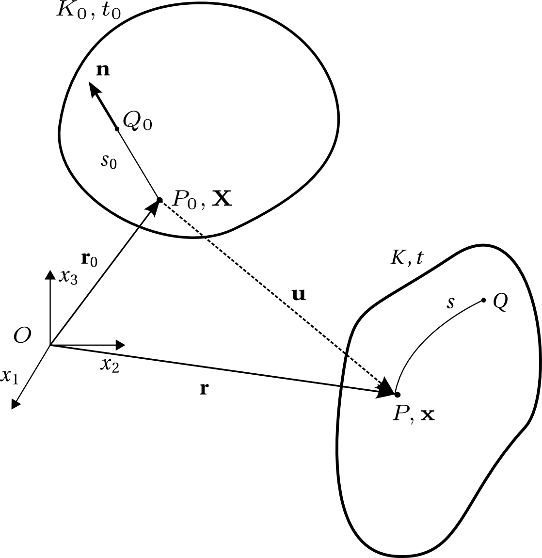
In Figure 17 a body is represented in the current configuration $K$ at time $t$ and in the reference configuration $K_0$ at time $t_0$. The position of an arbitrary particle, denoted $P$, in the body in the current configuration $K$ is given by $\boldsymbol{r}(\boldsymbol{r}_0,t)$, where $\boldsymbol{r}_0$ is the location of the same particle, denoted $P_0$, in the reference configuration $K_0$. The set of coordinates of $\boldsymbol{r}_0$ is conventionally denoted $X$ with corresponding spatial components $X_1,X_2,X_3$. The terms location and particle are used interchangeably for convenience, and thus we may refer to the particle $\boldsymbol{r}_0$ or the particle $X$.

The vector $\boldsymbol{r}(\boldsymbol{r}_0,t)$ is a function which represents the motion of an arbitrary particle in the body, which originally had the position $\boldsymbol{r}_0$. It may also be thought of as a map between the reference and current configuration. The motion may be represented as vector valued function or by its components: $$\begin{equation} \boldsymbol{r} = \boldsymbol{r}(\boldsymbol{r}_0,t) \Leftrightarrow x_i = x_i(X,t) \tag{3.1} \end{equation}$$

The displacement vector $\boldsymbol{u}(\boldsymbol{r}_0,t)$ (see Figure 17 ) is also a function which represents motion relative to the original location: $$\begin{equation} \boldsymbol{u}(\boldsymbol{r}_0,t) = \boldsymbol{r}(\boldsymbol{r}_0,t)-\boldsymbol{r}_0 \tag{3.2} \end{equation}$$

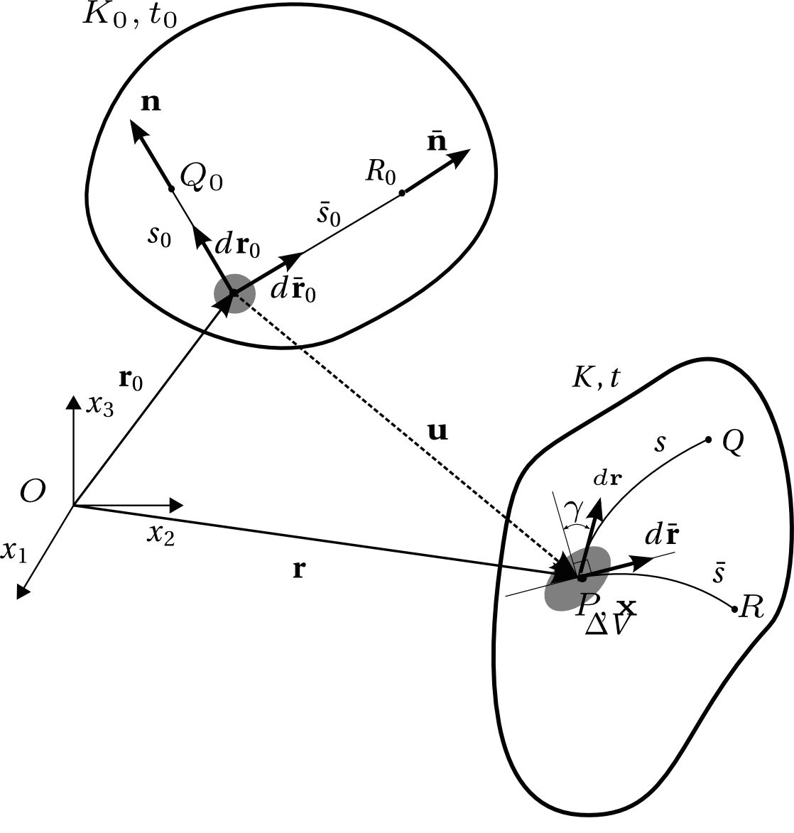
Let $P_0$ denote the point with coordinates $\bf{r}_0$ in$K_0$ Let $s_0=P_0Q_0$ denote the length the straight line from $P_0$ to $Q_0$ in the reference configuration $K_0$ from $\bf{r}_0$ in the direction of $\boldsymbol{n}$. In general this line will change both form and length in the current configuration $K$, where its length is represented by $s=PQ$. Definitions of the three measures strain may then be formulated:

Longitudinal strain $\epsilon$ The longitudinal strain $\epsilon$ in the direction $\boldsymbol{n}$ in a particle $\boldsymbol{r}_0$ is defined by: $$\begin{equation} \epsilon= \lim_{s_0 \rightarrow 0} \frac{s-s_0}{s_0} = \frac{d s - d s_0}{d s_0} = \frac{d s}{d s_0} -1 \tag{3.3} \end{equation}$$

The longitudinal strain $\epsilon$ represents the change of length per unit length in the direction of $\boldsymbol{n}$ in particle $\boldsymbol{r}_0$.

Figure 18 illustrates the same situation as in Figure 17, albeit with some more details, allowing for the definition of shear strain:

Shear strain $\gamma$ The angular deviation (in radians) from $\pi/2$ between two material lines in $K$ which originally were perpendicular in $K_0$. The shear strain $\gamma$, is taken to be positive when the angle is reduced.

In Figure 18, the shear strain $\gamma$ is illustrated at the location $\mathbf{r}_0$, as the angular deviation from $\pi/2$ between $\mathbf{n}$ and $\mathbf{\bar{n}}$, two perpendicular material line elements in the reference configuration $K_0$.

Volumetric strain $\epsilon_v$ $$\begin{equation} \epsilon _v = \mathop {\lim }\limits_{\Delta V_0 \to 0} \frac{{\Delta V - \Delta V_0 }}{{\Delta V_0 }} \tag{3.4} \end{equation}$$

The volumetric strain $\epsilon_v$ represents change in a differential volume per unit undeformed differential volume around the particle $\boldsymbol{r}_0$.

In the following, commonly used expressions for the primary measures of strain will be introduced.

• «
• 1
• 2
• 3
• 4
• 5
• 6
• 7
• 8
• 9
• 10
• 11
• 12
• 13
• 14
• 15
• 16
• 17
• 18
• ...
• 43
• »